Day 7
MATH 313: Survey Design and Sampling
Simple Random Sampling
Definition
If a sample of size \(n\) is drawn from a population of size \(N\) such that every possible sample of size \(n\) has the same chance of being selected, then the sampling procedure is called simple random sampling. The sample thus obtained is called a simple random sample.
How to Draw a Simple Random Sample
To draw a simple random sample, number every item \((1, 2, \ldots, N)\) in the population and select a list of \(n\) non-repeated random numbers within \(1, 2, \ldots, N\).
- In the lab, we saw how to generate such a list using R.
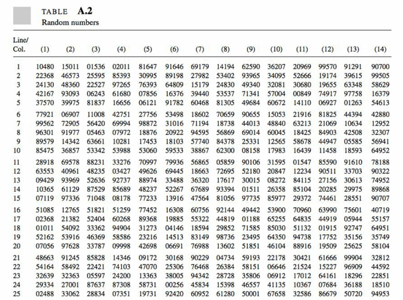
- We can also use a random number table (textbook Appendix A, Table A.2).

Example 1: Use the random number table, select a random sample with size 5 from a population with \(N=20\). use the rightmost digit on the \(15^{th}\) line and \(9^{th}\) column as the starting point.
Example 2: Use the random number table, select a random sample with size 10 from the list of States in U.S.A. Use the last two digit on the \(10^{th}\) line and \(9^{th}\) column as the starting point.
Estimation Using Simple Random Sampling
- Population Mean (\(\mu\)): Estimated using the sample mean.
- Population Total (\(\tau\)): Estimated using the product of mean and population size.
\[\bar{y} = \frac{1}{n} \sum_{i=1}^n y_i\] \[\hat{\tau} = N \cdot \bar{y}\]
Variance Estimates in Sampling
Variance of the Sample Mean (\(V(\bar{y})\)):
- The variance is calculated using: \[ V(\bar{y}) = \frac{\sigma^2}{n} \left(\frac{N-n}{N-1}\right) \]
- Adjusted for finite population: \[ = \left(1 - \frac{n}{N}\right) \frac{s^2}{n} \]
Sample Variance (\(s^2\)): \[ s^2 = \frac{1}{n-1} \sum (y_i - \bar{y})^2 \]
Expectation of Sample Variance: \[ E(s^2) = \frac{N}{N-1} \cdot \sigma^2 \]
Variance of Estimated Total (\(V(\hat{\tau})\))
- Adjusted for scaling by the population size: \[ V(\hat{\tau}) = N^2 \cdot V(\bar{y}) \]
- Which results in: \[ = N^2 \cdot \left(1 - \frac{n}{N}\right) \frac{s^2}{n} \]
Constructing Confidence Intervals
For both the population mean (\(\mu\)) and total (\(\tau\)), use the respective variance calculations to construct confidence intervals, accounting for the finite population correction.
- This approach ensures more accurate estimations by adjusting for the finite size of the population.
Note: When the population variance \(\sigma^2\) is unknown, we use \(s^2\) as an estimator. However, to account for the finite population size, the sample variance \(s^2\) should be multiplied by \(\frac{N-1}{N}\) to make it an unbiased estimator of \(\sigma^2\). This scaling helps adjust the variance estimate to reflect the true variability in the population more accurately.
Example 3: The census population of each states in U.S.A in 2020 is listed below. Use the simple random sample we obtained in Example 2, estimate the average census population, \(\bar{y}\) of a state in the U.S.A., then compute the estimated variance of \(\bar{y}\). Do the same computation for the total census population for the whole 50 states.