Day 37
MATH 313: Survey Design and Sampling
Stocked Quadrat Sampling Method
Stocked quadrat sampling efficiently determines species presence within plots, simplifying data collection. This method involves counting quadrats as either stocked or unstocked based on species presence, simplifying statistical analysis but requiring careful handling due to binary outcomes.
- Data Type: Presence or absence of species.
- Statistical Modeling: Often involves logistic regression or similar models.
Poisson Distribution in Ecological Sampling
Ecological counts are modeled using the Poisson distribution under the assumption that species are randomly distributed.
Key Concepts
- Modeling Assumption: Each quadrat’s count follows a Poisson distribution.
- Expected Counts: \(\lambda a\), where \(\lambda\) is the species density per unit area.
- Unstocked Probability: \[ P(\text{No individuals}) = e^{-\lambda a} \] This probability is crucial for estimating species density from unstocked quadrats.
Estimating Density from Unstocked Quadrats
Using the proportion of unstocked quadrats, we can estimate population density efficiently, which is especially useful in large ecological studies where direct counting is impractical.
- Estimator: \[ \hat{\lambda} = -\frac{1}{a} \ln\left(\frac{y}{m}\right) \]
Variance Estimation
- Density Variance: \[ \hat{V}(\hat{\lambda}) = \frac{1}{m a^2} \left(e^{\hat{\lambda} a} - 1\right) \]
- Population Variance: \[ \hat{V}(\hat{N}) = A^2 \hat{V}(\hat{\lambda}) = \frac{A^2}{m a^2} \left(e^{\hat{\lambda} a} - 1\right) \]
Derivations of \(\hat{V}(\hat{\lambda}\)) (Supplementary)
To derive the variance of \(\hat{\lambda}\) using the delta method, we start from the estimator:
\[ \hat{\lambda} = -\frac{1}{a} \ln\left(\frac{y}{n}\right) \]
Defining a transformation function \(g(x) = -\frac{1}{a} \ln(x)\), the delta method approximates the variance of \(\hat{\lambda}\) as:
\[ \hat{V}(g(X)) \approx [g'(E(X))]^2 \hat{V}(X) \]
where \(X = \frac{y}{m}\) and \(E(X) = e^{-\lambda a}\). Calculating the derivative \(g'(x)\):
\[ g'(x) = -\frac{1}{a} \cdot \frac{1}{x} \]
Plugging in \(E(X) = e^{-\lambda a}\):
\[ g'(E(X)) = -\frac{1}{a} e^{\lambda a} \]
Assuming \(X\) follows a binomial distribution, the variance of \(X\) is:
\[ \hat{V}(X) = \frac{E(X)(1 - E(X))}{m} = \frac{e^{-\lambda a}(1 - e^{-\lambda a})}{m} \]
Substituting back into the delta method formula:
\[ \hat{V}(\hat{\lambda}) = \left(-\frac{1}{a} e^{\lambda a}\right)^2 \cdot \frac{e^{-\lambda a}(1 - e^{-\lambda a})}{m} = \frac{1}{m a^2} \left(e^{\lambda a} - 1\right) \]
Example 1: To estimate the density and total number of trees having fusiform rust on a southern-pine plantation of 200 acres, \(m=20\) quadrats of 0.5 acre each will be sampled, but only the presence or absence of infected trees will be noted for each sampled quadrat. (Because this task is easier than counting trees, the sample size can be increased.) Suppose \(y=4\) of the 20 quadrats show no signs of fusiform rust. Estimate the density and the total number of infected trees, placing a 95% bounds on the error of estimation in both cases.
Introduction to Adaptive Sampling
Adaptive sampling adjusts the sampling strategy based on findings during data collection, enhancing the efficiency of estimating population densities, especially in clustered distributions like forests.
Concept
- Adaptive Technique: Explores neighboring cells if a species is detected, leveraging the spatial cluster tendency of species like maple trees.
- Implementation: Begins with a regular grid over a study area; expands sampling dynamically as species are detected.
Adaptive Sampling Strategy and Estimation
This sampling method allows researchers to intensify their sampling efforts in promising areas, potentially reducing overall effort while increasing accuracy.
Process
- Sampling Growth: If species are detected in a sampled cell, adjacent cells are also sampled, continuing until no new species are found in the surrounding cells.
- Density Estimation: \[ \hat{\mu}=\frac{1}{m} \sum_{i=1}^{m} \frac{y_{i}}{m_{i}}=\frac{1}{m} \sum_{i=1}^{m} \bar{y}_{i} \] This approach estimates the mean density per cell, applying corrections for the adaptive sampling design.
Variance Calculation
Variance Estimation: \[ \hat{V}(\hat{\mu})=\left(1-\frac{m}{M}\right) \frac{s_{\bar{y}}^{2}}{m} \] where \(s_\bar{y}^2=\frac{\sum_{i=1}^m\left(\overline{y_i}-\hat{\mu}\right)^2}{m-1}\)
Reflects the increased precision of adaptive sampling over simple random sampling.
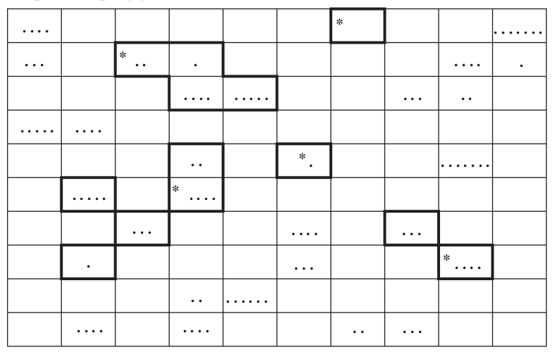
Example 2: Back to our forest, maple trees, and the grid pictured in the following Figure. Suppose a random sample of \(m=5\) of the \(M=100\) cells is selected and the asterisks \((*)\) mark the five that come up in a simple random sample. The adaptive sampling scheme is added onto this original sample as follows. If a sampled cell has at least one maple tree in it, then the eight neighboring cells (East, SE, South, SW, West, NW, North, and NE)are investigated as well. If any one of those cells contains a maple tree, it is added to the sample and its neighboring cells are investigated. The process continues until the cell network is surrounded by cells devoid of maple trees.
