Day 28

MATH 313: Survey Design and Sampling

Bastola

Comprehensive Guide to Cluster Sampling

Cluster Sampling emerges as a cost-effective and efficient sampling design, particularly advantageous in scenarios where a full listing of population elements is impractical or overly expensive. This sampling method is instrumental in gathering substantial information with minimized resource expenditure.

Key Concepts and Benefits

Cost Reduction: By sampling clusters (e.g., city blocks or regions), rather than individual units (e.g., households), significant savings on logistical and operational costs are achieved, especially when geographical dispersion of the population elements is a factor.
Feasibility: The necessity for a detailed frame listing all elements is circumvented, allowing for practical implementation in large-scale surveys or studies.

Implementation Steps in Cluster Sampling

Cluster sampling involves several key steps, each critical to the success of the sampling strategy. These steps are defined with precise terminology to ensure clarity and accuracy.

Identify Clusters: Divide the population into natural clusters, referred to as \(M\), where \(M\) is the total number of clusters in the population.
Determine Sample Size: Decide on the number of clusters, \(m\), to sample randomly. Each cluster \(i\) contains \(n_i\) elements, contributing to the determination of cluster sizes.
Random Selection: Randomly select \(m\) clusters from the population. This step ensures that each cluster has an equal chance of being included in the sample.
Data Collection: Collect data from every element within each chosen cluster. The total of observations within the \(i^{th}\) cluster is represented by \(\tau_i\), and each observation in the cluster is indexed by \(j\) (denoted \(y_{i j}\)).
Statistical Calculation: Calculate the average cluster size for the sample as \(\frac{1}{m} \cdot \sum_{i=1}^m n_i\), and for the population as \(\bar{N} = \frac{N}{M}\), where \(N = \sum_{i=1}^M n_i\) represents the total population size.

Design Considerations

Cluster Homogeneity: Unlike strata, which should be as homogeneous as possible to minimize variance within each stratum, clusters should be internally heterogeneous but similar to each other to maximize the representativeness of the sample. This configuration enhances the accuracy of the estimates derived from the sample.

Practical Application Example

Imagine estimating the average income per household in a large city. Cluster sampling allows selecting city blocks as clusters and surveying every household within those blocks, thereby reducing the cost and complexity of the sampling process.

Strategic Advantages

Reduced Travel Expenses: By concentrating the survey within geographical clusters, travel time and related costs for surveyors are significantly lowered.
Ease of Sampling: Using a frame that lists clusters (like city blocks), rather than individual households, simplifies the sampling process and enhances operational efficiency.

This method not only aligns with the objectives of minimizing costs and simplifying logistics but also adapts flexibly to various survey environments, proving essential for researchers and organizations aiming for efficient data collection strategies.

Estimating the Population Mean with Cluster Sampling

The population mean, \(\mu\), is estimated using a ratio estimator derived from sampled clusters. This approach leverages the proportional representation of each cluster to approximate the overall population mean.

Ratio Estimator Formula

\[ \bar{y} = \frac{\sum_{i=1}^{m} \tau_i}{\sum_{i=1}^{m} n_i} \] where \(\tau_i\) is the total of all observations within the \(i^{th}\) cluster, and \(n_i\) is the number of elements in the \(i^{th}\) cluster.

Calculation of Variance in Cluster Sampling

Estimating the variance of the population mean estimator is critical for assessing the precision of the sampling strategy.

Variance Formula

The estimated variance of the mean estimator \(\bar{y}\) is given by: \[ \hat{V}(\bar{y}) = \left(1-\frac{m}{M}\right) \frac{s_{\mathrm{r}}^2}{m\bar{N}^2} \] where \(s_{\mathrm{r}}^2 = \frac{\sum_{i=1}^m\left(\tau_i-\bar{y} n_i\right)^2}{m-1}\) is the residual sum of squares from the ratio estimation.

Confidence Intervals for Cluster Sampling

Constructing a confidence interval around \(\bar{y}\) helps quantify the uncertainty of our estimate.

Normal Approximation

For sufficiently large \(m\), typically \(m > 20\), the sampling distribution of \(\bar{y}\) can be approximated by a normal distribution, facilitating the computation of confidence intervals.

Confidence Interval Calculation

\[ \bar{y} \pm z \cdot \sqrt{\hat{V}(\bar{y})} \] where \(z\) is the z-score corresponding to the desired confidence level (e.g., 1.96 for 95% confidence).

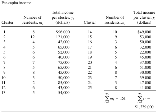
Example 1: A sociologist wants to estimate the per-capita income in a certain small city. No list of resi- dent adults is available. So she performed cluster sampling. The city is marked off into rectangular blocks, except for two industrial areas and three parks that contain only a few houses. The sociologist decides that each of the city blocks will be considered one cluster, the two industrial areas will be considered one cluster, and finally, the three parks will be considered one cluster. The clusters are numbered on a city map, with the numbers from 1 to 415.The experimenter has enough time and money to sample clusters and to interview every household within each cluster. Hence, 25 random numbers between1 and 415 are selected, and the clusters having these numbers are marked on the map.Interviewers are then assigned to each of the sampled clusters. The data on incomes are presented in the following. Use the data to estimate the per-capita income in the city and place a bound on the error of estimation.