Day 27

MATH 313: Survey Design and Sampling

Bastola

Welcome to Repeated Systematic Sampling

Today, we delve deeper into an advanced statistical technique—Repeated Systematic Sampling. Building on your understanding of systematic sampling, this method enhances the accuracy and reliability of our estimates by incorporating multiple starting points across the sampling frame.

Why does this matter? Even though systematic sampling is efficient, it doesn’t always equate to simple random sampling, potentially leading to biases. Repeated systematic sampling addresses this issue by averaging multiple systematic samples, thus approximating the randomness and reducing bias.

What will you learn?

• The setup for repeated systematic sampling, including choosing multiple starting points.
• Detailed formulas for estimating population mean and variance using repeated samples.
• Practical application: Calculating accurate estimates for variables like average visitors per car in a systematic manner.

Repeated Systematic Sampling Procedure

Repeated systematic sampling improves estimation reliability by utilizing multiple starting points. Here’s how we execute this method within a population of \(N\) elements:

• Step 1: Calculate the interval \(k=\frac{N}{n}\), defining the spacing between selected elements.
• Step 2: Set the number of samples, \(n_s\), typically 10 for comprehensive coverage.
• Step 3: Determine the extended interval \(k' = k \cdot n_s\), adjusting for multiple samples.
• Step 4: Randomly select \(n_s\) starting points from 1 to \(k'\).
• Step 5: From each starting point, conduct 1-in-\(k'\) sampling to capture diverse data points.
• Step 6: Aggregate all individual samples to form the complete systematic sample.

This approach systematically covers the population, ensuring each segment is represented, minimizing bias and enhancing the robustness of your results.

Estimation of Population Mean

The estimator of the population mean \(\mu\), using \(n_s\) systematic samples, is calculated with an emphasis on ensuring each sample contributes to a more reliable estimate:

\[ \hat{\mu}=\sum_{i=1}^{n_s} \bar{y}_i \cdot \frac{1}{n_s} \]

Here, \(\bar{y}_i\) represents the mean of the \(i^{th}\) systematic sample.

Variance Estimation

The variance of the estimated mean \(\hat{\mu}\) is crucial for understanding the spread and reliability of our estimate across different systematic samples. It is calculated as follows:

\[ S_{\bar{y}}^2=\frac{\sum_{i=1}^{n_s}\left(\overline{y_i}-\hat{\mu}\right)^2}{n_s-1} \]

\[ \hat{V}(\hat{\mu})=\left(1-\frac{n}{N}\right) \cdot \frac{S_{\bar{y}}^2}{n_s} \]

This formula helps quantify the uncertainty in our estimate, adjusting for the sample size relative to the population.

Estimation of Population Total

Using repeated systematic sampling, the population total \(\tau\) can be estimated from the means of the systematic samples, adjusted for the population size:

\[ \hat{\tau}=N \cdot \hat{\mu}=\frac{N}{n_s} \cdot \sum_{i=1}^{n_s} \bar{y}_i \]

To understand the reliability of this estimation, the variance of \(\hat{\tau}\) is also calculated, using the variance of \(\hat{\mu}\) scaled by the square of the population size:

\[ \hat{V}(\hat{\tau})=N^2 \cdot \hat{V}(\hat{\mu})=N^2\left(1-\frac{n}{N}\right) \cdot \frac{S_{\bar{y}}^2}{n_s} \]

Here, \(S_{\bar{y}}^2\) is calculated as \(\frac{\sum_{i=1}^{n_s}\left(\overline{y_i}-\hat{\mu}\right)^2}{n_s-1}\), reflecting the dispersion within and across the systematic samples.

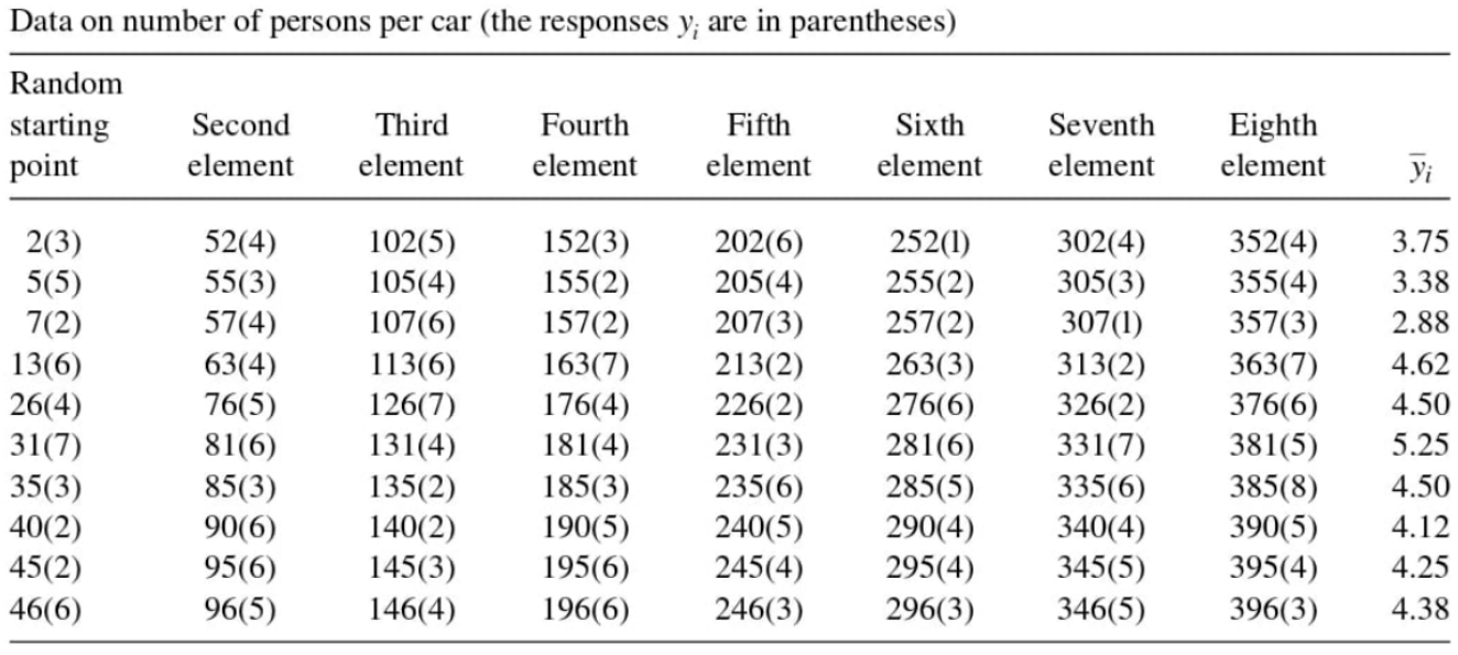
Example 1: A state park charges admission by carload rather than by person, and a park official wants to estimate the average number of people per car for a particular summer holiday. She knows from past experience that there should be approximately 400 cars entering the park, and she wants to sample 80 cars. To obtain an estimate of the variance, she uses repeated systematic sampling with ten samples of eight cars each. Using the data given in the following table, estimate the average number of people per car and place a 95% bound on the error of estimation.