Day 24
MATH 313: Survey Design and Sampling
Introduction to Estimators
In survey sampling, different estimators provide various ways to estimate population parameters. Today, we will explore:
- Simple Random Sampling Estimator (\(\bar{y}\))
- Ratio Estimator (\(\hat{\mu}_{y}\))
- Regression Estimator (\(\hat{\mu}_{y L}\))
- Difference Estimator (\(\hat{\mu}_{y D}\))
Each estimator has unique properties and use cases.
Understanding Bias in Estimators
Bias refers to the difference between an estimator’s expected value and the true value of the population parameter:
- Simple Sampling (\(\bar{y}\)): Always unbiased.
- Ratio Estimator (\(\hat{\mu}_{y}\)): Biased except under specific conditions.
- Regression Estimator (\(\hat{\mu}_{y L}\)): Biased for finite populations unless the data points are linear.
- Difference Estimator (\(\hat{\mu}_{y D}\)): Always unbiased.
Key Note: Bias affects how we interpret and trust our estimations.
Relative Efficiency
Relative Efficiency (RE) helps compare two estimators based on their variances under similar conditions:
- Higher RE (>1) means the first estimator is generally better (lower variance).
- Lower RE (<1) favors the second estimator.
\[ \text{RE}(T_1, T_2) = \frac{\hat{V}(T_2)}{\hat{V}(T_1)} \]
RE is crucial when deciding which estimator provides the most reliable results.
Estimator Performance Comparison
| Estimator | Estimated Mean | Estimated Variance | 95% CI |
|---|---|---|---|
| Simple Random Sampling | \(\mu_{y}\) | \(\hat{V}(\bar{y})\) | \(\mu_{y} \pm t_{1-\alpha/2, \text{df}} \sqrt{\hat{V}(\bar{y})}\) |
| Ratio Estimator | \(\hat{\mu}_{y}\) | \(\hat{V}(\hat{\mu}_{y})\) | \(\hat{\mu}_{y} \pm t_{1-\alpha/2, \text{df}} \sqrt{\hat{V}(\hat{\mu}_{y})}\) |
| Regression Estimator | \(\hat{\mu}_{y L}\) | \(\hat{V}(\hat{\mu}_{y L})\) | \(\hat{\mu}_{y L} \pm t_{1-\alpha/2, \text{df}} \sqrt{\hat{V}(\hat{\mu}_{y L})}\) |
| Difference Estimator | \(\hat{\mu}_{y D}\) | \(\hat{V}(\hat{\mu}_{y D})\) | \(\hat{\mu}_{y D} \pm t_{1-\alpha/2, \text{df}} \sqrt{\hat{V}(\hat{\mu}_{y D})}\) |
Each estimator uses the sample to provide different insights into the population’s characteristics.
Visualizing Data Relationships
Plot Analysis:
- A strong linear relationship suggests the use of a regression or ratio estimator.
- Non-linear relationships may require more complex models or the difference estimator for better accuracy.
Choosing the Right Estimator
Deciding factors:
- Linearity and Bias: If data points are linear, regression and ratio estimators are effective.
- Relative Efficiency: Higher RE indicates a more efficient estimator under given conditions.
- Unbiased Nature: Preference for unbiased estimators in settings where bias can’t be controlled.
Practical examples and simulations help in understanding estimator performance.
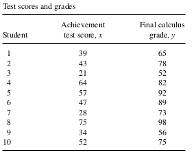
Example 1 A mathematics achievement test was given to 486 students prior to their entering a certain college. From these students a simple random sample of \(n=10\) students was selected and their progress in calculus observed. Final calculus grades were then reported, as given in the following table. It is known that \(\mu_x=52\) for all 486 students taking the achievement test. Estimate \(\mu_y\) for this population (estimator value, estimated variance, \(95 \%\) bound on error, and \(95 \%\) confidence interval). Use the simple random sampling estimator, ratio estimator, regression estimator, and difference estimator, and perform comparisons.
