Day 23

MATH 313: Survey Design and Sampling

Bastola

Difference Estimator of \(\mu_y\)

• The Difference Estimation method adjusts the sample mean \(\bar{y}\) by a value dependent on the difference \((\mu_x - \bar{x})\).
• This method is akin to a special case of regression where the regression coefficient \(b\) is set to 1, simplifying the estimation process.

Assumptions and Methodology

• Assume a linear relationship without a slope component: \(y = x + a\).
• Thus, any change in \(x\) directly translates to a change in \(y\): \[ \mu_y - \bar{y} = \mu_x - \bar{x} \]

Formulation of the Difference Estimator

• The difference estimator for the population mean \(\mu_y\) is: \[ \hat{\mu}_{y D} = \bar{y} + (\mu_x - \bar{x}) = \mu_x + (\bar{y} - \bar{x}) \]
• Here, \(\bar{d} = \bar{y} - \bar{x}\) represents the average difference between the variables.

Variance of the Difference Estimator

• The estimated variance of \(\hat{\mu}_{y D}\) is given by: \[ \hat{V}(\hat{\mu}_{y D}) = \left(1-\frac{n}{N}\right) \cdot \left(\frac{1}{n}\right) \cdot \frac{\sum_{i=1}^n\left(y_i - x_i - \bar{d}\right)^2}{(n-1)} \]
• This accounts for the sampling variability and the differences between the paired observations.

Error Bounds and Confidence Interval

• \((1-\alpha) \times 100\%\) bound on the error of estimation: \[ B = t_{1-\frac{\alpha}{2}, (n-1)} \cdot \sqrt{\hat{V}(\hat{\mu}_{y D})} \]
• Confidence Interval for \(\hat{\mu}_{y D}\): \[ \hat{\mu}_{y D} \pm B \]
• This interval estimates where the true mean \(\mu_y\) lies with \((1-\alpha) \times 100\%\) confidence.

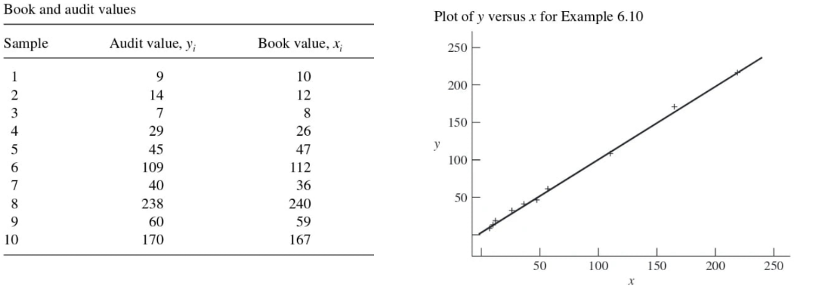
Example 1: Auditors are often interested in comparing the audited value of items with the bookvalue. Generally, book values are known for every item in the population, and auditvalues are obtained for a sample of these items. The book values can then be used toobtain a good estimate of the total or average audit value for the population. Suppose a population contains 180 inventory items with a stated book value of \(\$ 13,320\). Let \(x_i\) denote the book value and \(y_i\) the audit value of the \(i\) th item. A simple random sample of items yields the results shown in the following table. A plot of these data shows them to lie along a straight line through the origin, with a slope fairly close to 1 . Estimate the mean audit value of \(\mu_y\) by the difference method for this population (estimator value, estimated variance, \(95 \%\) bound on error, and \(95 \%\) confidence interval).