Day 22
MATH 313: Survey Design and Sampling
Bastola
Regression Estimator of \(\mu_y\)
- Use regression estimator when there is evidence of a linear relationship between \(y\) and \(x\), without the restriction of passing through the origin.
- Essential for situations where the auxiliary variable \(x\) provides valuable information for estimating the mean \(\mu_y\).
Assumptions
- Linear relationship modeled as: \[ y_i = a + b x_i + \varepsilon_i \]
- Where \(\varepsilon_i\) represents random errors which we assume have a mean of zero and are independent of \(x_i\).
Estimation without the Error Term
- Ignoring the error, the predicted value of \(y_i\): \[ \hat{y}_i = \bar{y} + b (x_i - \bar{x}) \]
- Coefficient \(b\), known as the slope of the regression line, is given by: \[ b = \frac{\sum_{i=1}^n [(y_i - \bar{y})(x_i - \bar{x})]}{\sum_{i=1}^n (x_i - \bar{x})^2} \]
Regression Estimator for Population Mean \(\mu_y\)
- The regression estimator for the population mean is: \[ \hat{\mu}_{y L} = \bar{y} + b(\mu_x - \bar{x}) \]
- This estimator adjusts the sample mean \(\bar{y}\) for the deviation of the expected value of \(x\) from its sample mean, scaled by the regression coefficient \(b\).
Variance of the Regression Estimator
- The variance of \(\hat{\mu}_{y L}\) is estimated as: \[ \hat{V}(\hat{\mu}_{y L}) = \left(1 - \frac{n}{N}\right) \left(\frac{1}{n}\right) \left(\frac{\sum_{i=1}^n (y_i - (\bar{y} + b (x_i - \bar{x})))^2}{n-2}\right) \]
Error Bounds and Confidence Interval
- The \((1-\alpha) \times 100\%\) bound on the error of estimation is calculated using: \[ B = t_{1-\frac{\alpha}{2}, n-2} \cdot \sqrt{\hat{V}(\hat{\mu}_{y L})} \]
- Consequently, the confidence interval for \(\hat{\mu}_{y L}\) is: \[ \hat{\mu}_{y L} \pm B \]
- This interval offers a range within which the true population mean is expected to lie with \((1-\alpha) \times 100\%\) confidence.
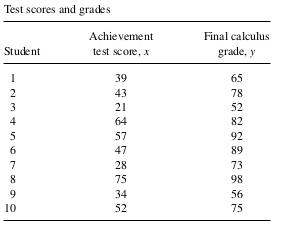
Example 1: A mathematics achievement test was given to 486 students prior to their entering a certain college. From these students a simple random sample of tudents was selected and their progress in calculus observed. Final calculus grades were then reported, as given in the following table. It is known that \(\mu_x=52\) for all 486 students taking the achievement test. Estimate \(\mu_y\) for this population (estimator value, estimated variance, \(95 \%\) bound on error, and \(95 \%\) confidence interval).
