Day 20

MATH 313: Survey Design and Sampling

Bastola

Correlation Coefficient \(\hat{\rho}\)

Measures the linear relationship strength between two variables.
Estimated using the Pearson method by default:

# Use R's cor() function for Pearson correlation
cor(X, Y)  # X and Y are numeric vector

Calculation of Covariance and Standard Deviations

Formulae for covariance and standard deviations:

\[ s_{xy} = \frac{1}{n-1} \sum_{i=1}^n\left(x_i-\bar{x}\right)\left(y_i-\bar{y}\right) \]

\[ s_x^2 = \frac{1}{n-1} \sum_{i=1}^n\left(x_i-\bar{x}\right)^2 \]

\[ s_y^2 = \frac{1}{n-1} \sum_{i=1}^n\left(y_i-\bar{y}\right)^2 \]

Coefficient of Variation (CV)

Represents the ratio of the standard deviation to the mean.
Provides a standardized measure of dispersion of a probability distribution or frequency distribution.

Motivation for using CV:

Unlike the standard deviation, the coefficient of variation is unitless. This makes it especially useful when comparing data with different units or vastly different mean values.

# Calculate Coefficient of Variation for two variables X and Y
cv_x <- sd(X) / mean(X)
cv_y <- sd(Y) / mean(Y)

Large-Sample Confidence Interval for Ratio \(R\)

Approximate \(90\%\) confidence interval for \(R\):

\[ r \pm 1.645 \sqrt{\hat{V}(r)} \]

Where \(\hat{V}(r)\) is the estimated variance of \(r\), in terms of \(\hat{\rho}\):

\[ \hat{V}(r) = \frac{1-f}{n} r^2 \left((\operatorname{cv}(y))^2 + (\operatorname{cv}(x))^2 - 2 \hat{\rho} \cdot \operatorname{cv}(x) \cdot \operatorname{cv}(y)\right) \]

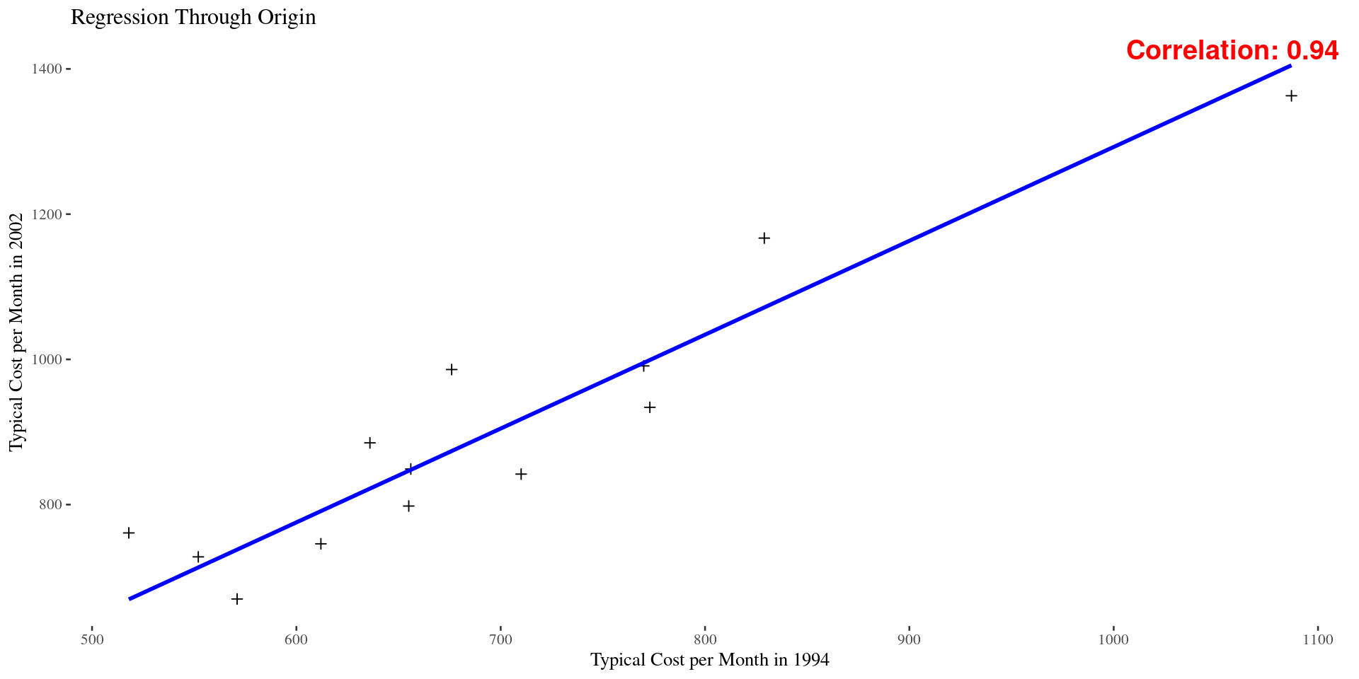
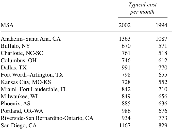
Example 1: The U.S. government’s American Housing Survey keeps tabs on many aspects of the characteristics of housing in America, including monthly costs for home ownership and the value of houses. One aspect of the survey tracks 47 metropolitan statistical areas (MSAs) over time by sampling a subset of them every four years or so. The survey for 2002 sampled the 13 MSAs listed in Table 6.1. Also listed there are the typical monthly costs of home ownership (not including maintenance) for 2002 and 1994 as well as the typical values of houses in those two years, respectively. These data are for owner-occupied houses only. Use these data to estimate \(R\), the ratio of mean typical monthly costs for 2002 as compared to those of 1994 for all 47 MSAs and calculate an appropriate margin of error.

Scatter-plot
Code

costs <- data.frame(
  MSA = c("Anaheim-Santa Ana, CA", "Buffalo, NY", "Charlotte, NC-SC", "Columbus, OH",
          "Dallas, TX", "Fort Worth-Arlington, TX", "Kansas City, MO-KS", "Miami-Fort Lauderdale, FL",
          "Milwaukee, WI", "Phoenix, AS", "Portland, OR-WA", "Riverside-San Bernardino-Ontario, CA", "San Diego, CA"),
  X1994 = c(1087, 571, 518, 612, 770, 655, 552, 710, 656, 636, 676, 773, 829),
  X2002 = c(1363, 670, 761, 746, 991, 798, 728, 842, 849, 885, 986, 934, 1167)
)

correlation_coefficient <- cor(costs$X1994, costs$X2002)

ggplot(costs, aes(x = X1994, y = X2002)) +
  geom_point(pch = 3) +  
  geom_smooth(method = "lm", formula = y ~ x - 1, se = FALSE, color = "blue") +
  labs(title = "Regression Through Origin and Specific Point",
       x = "Typical Cost per Month in 1994",
       y = "Typical Cost per Month in 2002") +
  annotate("text", x = Inf, y = Inf, label = sprintf("Correlation: %.2f", correlation_coefficient), 
           hjust = 1.05, vjust = 1.05, size = 5, color = "red", fontface = "bold", angle = 0)

Calculate an approximate \(90\%\) confidence interval for the ratio \(R\) using the correlation coefficient from the above example.

# Calculate means
mean_1994 <- mean(costs$X1994)
mean_1994

[1] 695.7692

mean_2002 <- mean(costs$X2002)
mean_2002

[1] 901.5385

# Calculate standard deviations
sd_1994 <- sd(costs$X1994)
sd_1994

[1] 148.479

sd_2002 <- sd(costs$X2002)
sd_2002

[1] 192.4784

# Calculate coefficients of variation
cv_1994 <- sd_1994 / mean_1994
cv_1994

[1] 0.2134027

cv_2002 <- sd_2002 / mean_2002
cv_2002

[1] 0.2134999

# Calculate the correlation coefficient
correlation <- cor(costs$X1994, costs$X2002)
correlation

[1] 0.9380038

# Set the assumed slope of the regression line through the origin
r <- mean_2002 / mean_1994
r

[1] 1.295744

# Sample size
n <- length(costs$X1994)
N <- 47

# Sampling fraction 
f <- n/N

# Variance calculation 
var_r <- ((1 - f) / n) * r^2 * (cv_2002^2 + cv_1994^2 - 
                              2 * correlation * cv_1994 * cv_2002)

# Calculate the confidence interval at 90% confidence level
ci <- r + c(-1,1)*qt(0.95, df = n)* sqrt(var_r)
ci

[1] 1.255058 1.336429